Patent and Solow Growth Panel Data
Data extraction via web, cleaning in Python and Econometric Analysis in R
Contents
This project serves as an opportunity for me to gain experience in Python for:
- data extraction via URL from OECD remotely
- data cleaning of large dataset from Penn World Data (PWT)
- data merging of two different sources into a workable penel dataset of 8 countryies.
Then, in a integrated work environment (RStudio), we export the extracted/filtered/cleaned/merged dataset into .cvs files to then analyze the data in R.
Results
Panel Dataset
Below are the final results of this project, which consist of the constructed panel dataset covering 8 countries from 1980–2019. The dataset integrates OECD patent data with Penn World Table macroeconomic indicators, cleaned and merged into a consistent format. It includes measures of output (GDP), capital, effective labor, total factor productivity (TFP), and patent activity, along with their computed growth rates. The full data, panel_complete.csv is displayed in the table below.
Besides the core panel dataset, I also generated panel_lags.csv, which adds one-, two-, and three-year lags of patent growth for fixed-effects regressions.
Time Series


Behind the Scenes (Complete Codes)
Python Data Extraction/Clean
OECD Data Set
library(reticulate)
library(dplyr)
library(ggplot2)
library(plm)
library(mFilter)
library(reticulate)
library(lmtest)
library(sandwich)
library(plm)
library(zoo)
library(broom)
library(reshape2)
library(ggrepel)
library(fixest)
We extract data from OECD remotely and PWT locally. First we set up our python
import pandas as pd
import numpy as np
import matplotlib.pyplot as plt
import requests
import xml.etree.ElementTree as ET
from io import StringIO
Now we extract data from filtered OECD data query.
url_data = (
    "https://sdmx.oecd.org/public/rest/data/"
    "OECD.STI.PIE,DSD_PATENTS@DF_PATENTS,1.0/"
    ".A.GR.PATN.PRIORITY.CAN+FRA+SGP+KOR+DEU+GBR+CHN+JPN+USA..INVENTOR.._Z._T"
    "?startPeriod=1980&endPeriod=2019&dimensionAtObservation=AllDimensions"
)

response_data = requests.get(url_data)
print("Status:", response_data.status_code)
## Status: 200
Parse into DataFrame (XML $\to$ Pandas)
root = ET.fromstring(response_data.text)
ns = {"generic": "http://www.sdmx.org/resources/sdmxml/schemas/v2_1/data/generic"}

records = []

for obs in root.findall(".//generic:Obs", ns):
    obs_dict = {}

    # Extract all keys (country, date type, etc.)
    for val in obs.findall("./generic:ObsKey/generic:Value", ns):
        obs_dict[val.attrib["id"]] = val.attrib["value"]

    # Extract the observed value
    val_elem = obs.find("./generic:ObsValue", ns)
    obs_dict["value"] = val_elem.attrib.get("value") if val_elem is not None else None

    records.append(obs_dict)

df_patents = pd.DataFrame(records)

print(df_patents.head())
##   TIME_PERIOD PATENT_AUTHORITIES  ... OECD_TECHNOLOGY_PATENT              value
## 0        2011                6F0  ...                     _T  3445.668701171875
## 1        2011                6F0  ...                     _T     14546.98828125
## 2        2000                6F0  ...                     _T    13811.802734375
## 3        2000                6F0  ...                     _T   14547.6337890625
## 4        2000                6F0  ...                     _T  851.2003784179688
##
## [5 rows x 13 columns]
print("Shape:", df_patents.shape)
## Shape: (720, 13)
We want REF_AREA, TIME_PERIOD, value
df_clean = df_patents[["REF_AREA", "TIME_PERIOD", "value"]].copy()
df_clean["TIME_PERIOD"] = df_clean["TIME_PERIOD"].astype(int)
df_clean["value"] = df_clean["value"].astype(float)

print(df_clean.head())
##   REF_AREA  TIME_PERIOD         value
## 0      KOR         2011   3445.668701
## 1      JPN         2011  14546.988281
## 2      DEU         2000  13811.802734
## 3      USA         2000  14547.633789
## 4      CAN         2000    851.200378
print("Shape:", df_clean.shape)
## Shape: (720, 3)
# Step 2a: aggregate by country + year (sum across authorities etc.)
df_agg = df_clean.groupby(["TIME_PERIOD", "REF_AREA"], as_index=False)["value"].sum()

# Step 2b: pivot to wide format
df_panel = df_agg.pivot(index="TIME_PERIOD", columns="REF_AREA", values="value")

print(df_panel.head())
## REF_AREA             CAN      CHN  ...      SGP           USA
## TIME_PERIOD                        ...
## 1980         1240.127747   5.0000  ...  15.4524  43367.697266
## 1981         1362.677399   3.1666  ...   5.3929  41946.530273
## 1982         1332.704742   3.0000  ...   3.7858  43240.144043
## 1983         1423.382584  11.3333  ...   5.5000  42562.730957
## 1984         1569.370361  11.2834  ...  16.7333  44211.058105
##
## [5 rows x 9 columns]
print("Shape:", df_panel.shape)
## Shape: (40, 9)
Check empty
print(df_panel.isna().sum())
## REF_AREA
## CAN    0
## CHN    0
## DEU    0
## FRA    0
## GBR    0
## JPN    0
## KOR    0
## SGP    0
## USA    0
## dtype: int64
Let’s peek at the data:
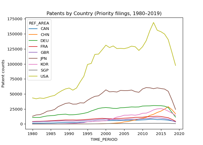
df_panel.plot(title="Patents by Country (Priority filings, 1980–2019)")
plt.xlabel("TIME_PERIOD")
plt.ylabel("Patent counts")
plt.show()
Looking good now we proceed similarly for our second data set.
PWT Data Set
Here we clean and extract data from Penn World Table We begin with understanding the data structure.
xls = pd.ExcelFile("pwt1001.xlsx")
print(xls.sheet_names)
## ['Info', 'Legend', 'Data']
# output ['Info', 'Legend', 'Data'];
df_legend = pd.read_excel("pwt1001.xlsx", sheet_name="Legend")
print("Variabe-Defn:")
## Variabe-Defn:
print(df_legend.head())
##           Variable name        Variable definition
## 0  Identifier variables                        NaN
## 1           countrycode  3-letter ISO country code
## 2               country               Country name
## 3         currency_unit              Currency unit
## 4                  year                       Year
For convenience let’s save this definition list for reference:
df_legend.to_csv("PWD_def", index = False)
print("def list saved as PWD_def.csv")
## def list saved as PWD_def.csv
After some considerations we will use:
- $Y_{i,t} :=$
rgdpo, i.e., Output-side real GDP at current PPPs (in mil. 2017US$). - $K_{i,t} :=$
rnna, i.e., Capital stock at constant 2017 national prices (in mil. 2017US$). - $L^{\text{effective}}_{i,t} \equiv$
emp$\times$avh$\times$hc, i.e., Number of persons engaged (in millions), Average annual hours worked by persons engaged, and the Human capital index. - $A_{i,t} :=$
rtfpna, i.e., TFP at constant national prices (2017=1).
Let’s have these variables filtered:
df_pwt = pd.read_excel("pwt1001.xlsx", sheet_name="Data")
df_pwt_small = df_pwt[[
    "countrycode", "year", "rgdpo", "rnna", "emp", "avh", "hc", "rtfpna"
]].copy()
print(df_pwt_small.head())
##   countrycode  year  rgdpo  rnna  emp  avh  hc  rtfpna
## 0         ABW  1950    NaN   NaN  NaN  NaN NaN     NaN
## 1         ABW  1951    NaN   NaN  NaN  NaN NaN     NaN
## 2         ABW  1952    NaN   NaN  NaN  NaN NaN     NaN
## 3         ABW  1953    NaN   NaN  NaN  NaN NaN     NaN
## 4         ABW  1954    NaN   NaN  NaN  NaN NaN     NaN
print(df_pwt_small.shape)
## (12810, 8)
In particular, we want the same countries as OECD dataset from 1980 to 2019:
keep_countries = ["CAN","CHN","DEU","FRA","GBR","JPN","KOR","SGP","USA"]

df_pwt_filtered = df_pwt_small[
    (df_pwt_small["countrycode"].isin(keep_countries)) &
    (df_pwt_small["year"].between(1980, 2019))
].copy()
print(df_pwt_filtered["countrycode"].unique())
## ['CAN' 'CHN' 'DEU' 'FRA' 'GBR' 'JPN' 'KOR' 'SGP' 'USA']
print(df_pwt_filtered["year"].min(), "→", df_pwt_filtered["year"].max())
## 1980 → 2019
print(df_pwt_filtered.shape)
## (360, 8)
Pivoting them:
# pivot each; I have deleted my testing process where I pint the head of each pivots
df_gdp = df_pwt_filtered.pivot(index="year", columns="countrycode", values="rgdpo")
df_cap = df_pwt_filtered.pivot(index="year", columns="countrycode", values="rnna")
df_pwt_filtered["eff_labour"] = df_pwt_filtered["emp"] * df_pwt_filtered["avh"] * df_pwt_filtered["hc"]
df_labor = df_pwt_filtered.pivot(index="year", columns="countrycode", values="eff_labour")
df_tfp = df_pwt_filtered.pivot(index="year", columns="countrycode", values="rtfpna")
# data from OECD set
df_patents_long = df_clean.rename(columns={
    "REF_AREA": "countrycode",
    "TIME_PERIOD": "year",
    "value": "patents"
})
df_patents_long["year"] = df_patents_long["year"].astype(int)
# merging
df_merged = pd.merge(
    df_pwt_filtered[["countrycode","year","rgdpo","rnna","eff_labour", "rtfpna"]],
    df_patents_long.groupby(["countrycode","year"], as_index=False)["patents"].sum(),
    on=["countrycode","year"],
    how="inner"
# name columns
)
df_merged = df_merged.rename(columns={
    "rgdpo": "Y",
    "rnna": "K",
    "eff_labour": "L",
    "rtfpna": "A",
    "patents": "PA"
})
print(df_merged.head())
##   countrycode  year            Y         K             L         A           PA
## 0         CAN  1980  687911.0625  0.272389  62465.899649  0.981520  1240.127747
## 1         CAN  1981  711280.5625  0.288998  64049.639423  0.979795  1362.677399
## 2         CAN  1982  693443.5000  0.299985  61399.551015  0.966170  1332.704742
## 3         CAN  1983  717049.3125  0.310637  62030.711466  0.973799  1423.382584
## 4         CAN  1984  767394.6875  0.321711  64472.861291  0.993447  1569.370361
print(df_merged.shape)
## (360, 7)
df_merged.to_csv("PWDnOECD.csv", index=False)
print("Saved as PWDnOECD.csv")
## Saved as PWDnOECD.csv
panel <- read.csv("PWDnOECD.csv")
head(panel)
##   countrycode year        Y         K        L         A       PA
## 1         CAN 1980 687911.1 0.2723894 62465.90 0.9815204 1240.128
## 2         CAN 1981 711280.6 0.2889977 64049.64 0.9797946 1362.677
## 3         CAN 1982 693443.5 0.2999851 61399.55 0.9661703 1332.705
## 4         CAN 1983 717049.3 0.3106366 62030.71 0.9737986 1423.383
## 5         CAN 1984 767394.7 0.3217106 64472.86 0.9934467 1569.370
## 6         CAN 1985 786765.8 0.3343326 67462.81 0.9967136 1565.460
We have thus completed our job in python. Now we move onto some elementary econometric analysis in R.
R Econometric Analysis
Time Series of the Data.
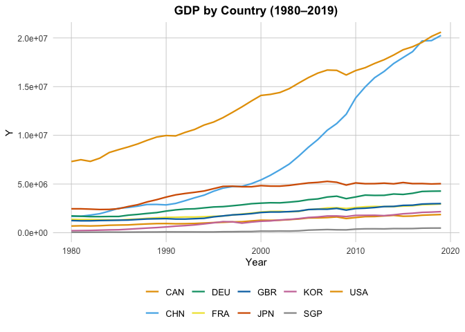
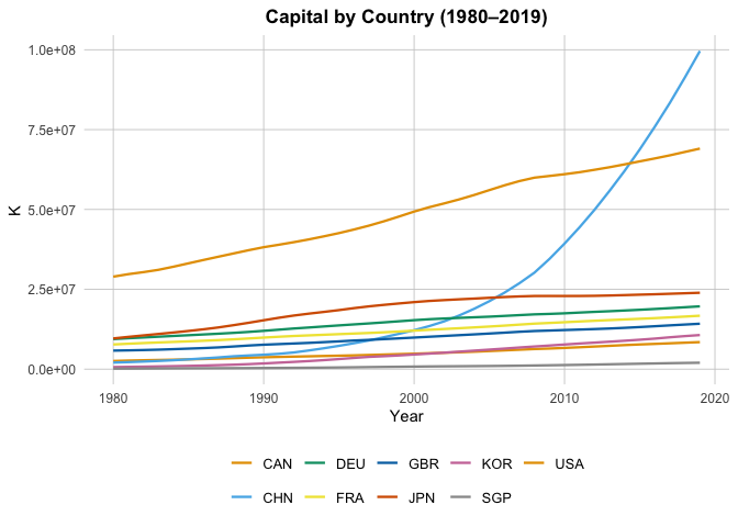
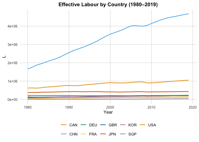
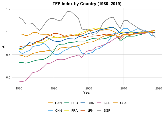
Let’s visualize and understand the time series trend of each of the variables:
okabe_ito <- c(
  "#E69F00", "#56B4E9", "#009E73", "#F0E442",
  "#0072B2", "#D55E00", "#CC79A7", "#999999"
)

variables <- c("Y", "K", "L", "A", "PA")
titles <- c(
  Y  = "GDP by Country (1980–2019)",
  K  = "Capital by Country (1980–2019)",
  L  = "Effective Labour by Country (1980–2019)",
  A  = "TFP Index by Country (1980–2019)",
  PA = "Patents by Country (1980–2019)"
)

for (var in variables) {
  p <- ggplot(panel, aes(x = year, y = .data[[var]], color = countrycode)) +
    geom_line(size = 0.8) +
    scale_color_manual(values = rep(okabe_ito, length.out = length(unique(panel$countrycode)))) +
    theme_minimal(base_size = 12) +
    labs(title = titles[[var]], x = "Year", y = var, color = "Country") +
    theme(
      legend.position = "bottom",
      legend.title = element_blank(),
      plot.title = element_text(size = 13, face = "bold", hjust = 0.5),
      axis.title = element_text(size = 11),
      axis.text = element_text(size = 9),
      panel.grid.minor = element_blank(),
      panel.grid.major = element_line(color = "grey80", size = 0.3)
    )
  print(p)
}
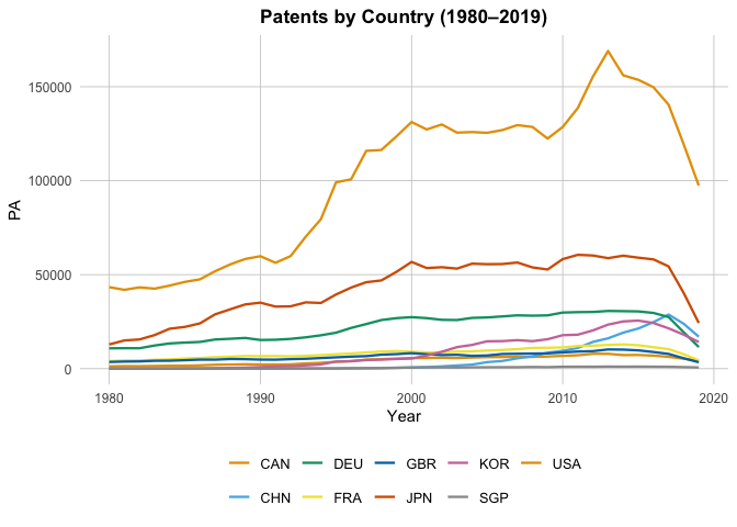
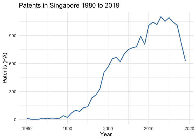
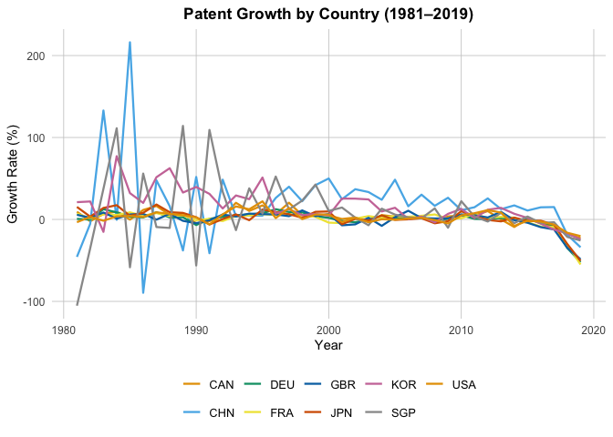
In particular, if we look at the Patents by Country plot, we can see the Singapore’s total patents nearly doesn’t grow. To look closer, we plot:
ggplot(panel[panel$countrycode == "SGP", ], aes(x = year, y = PA)) +
  geom_line(size = 1, color = "steelblue") +
  theme_minimal(base_size = 14) +
  labs(title = "Patents in Singapore 1980 to 2019",
       x = "Year", y = "Patents (PA)")
Growth Rate Time Series
Of course, we can further construct comparison of growth rate as follows:
mathematically speaking, we want for each variable $X$, \(gX_{i,t} = \ln(X_{i,t}) - \ln(X_{i,t-1}),\) which can be done easily with the ‘lag’ function:
panel_g <- panel %>%
  # 1) Make sure columns are numeric
  mutate(across(c(Y, K, L, A, PA), ~as.numeric(.))) %>%

  # 2) Sort properly
  arrange(countrycode, year) %>%

  # 3) Compute log-diff growths as percent
  group_by(countrycode) %>%
  mutate(
    gY   = 100 * c(NA, diff(log(Y))),
    gK   = 100 * c(NA, diff(log(K))),
    gL   = 100 * c(NA, diff(log(L))),
    gA   = 100 * c(NA, diff(log(A))),
    gPA  = 100 * c(NA, diff(log(PA)))
  ) %>%
  ungroup() %>%

  # 4) Keep only the growth-rate panel
  select(countrycode, year, gY, gK, gL, gA, gPA)

# for safety we now create a seperate dataset combining the two
panel_complete <- panel %>%
  left_join(panel_g, by = c("countrycode", "year"))
Quick check
ctry <- "CAN"

check <- panel_complete %>%
  filter(countrycode == ctry, year %in% c(1980, 1981)) %>%
  summarise(
    manual = 100 * (log(Y[year == 1981]) - log(Y[year == 1980])),
    stored = gY[year == 1981],
    equal  = all.equal(
      100 * (log(Y[year == 1981]) - log(Y[year == 1980])),
      gY[year == 1981]
    )
  )

print(check)
##     manual   stored equal
## 1 3.340739 3.340739  TRUE
Now by same logic we then have:
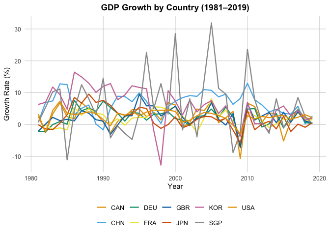
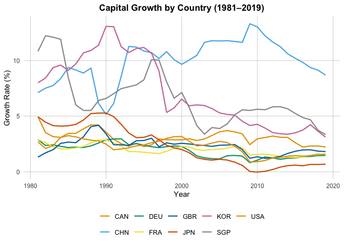
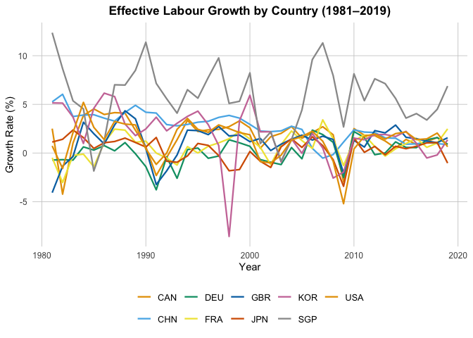
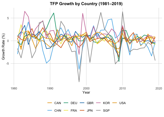
growth_vars <- c("gY", "gK", "gL", "gA", "gPA")
titles <- c(
  gY  = "GDP Growth by Country (1981–2019)",
  gK  = "Capital Growth by Country (1981–2019)",
  gL  = "Effective Labour Growth by Country (1981–2019)",
  gA  = "TFP Growth by Country (1981–2019)",
  gPA = "Patent Growth by Country (1981–2019)"
)

for (var in growth_vars) {
  p <- ggplot(panel_complete %>% filter(year >= 1981),
              aes(x = year, y = .data[[var]], color = countrycode)) +
    geom_line(size = 0.8) +
    scale_color_manual(values = rep(okabe_ito, length.out = length(unique(panel_complete$countrycode)))) +
    theme_minimal(base_size = 12) +
    labs(title = titles[[var]], x = "Year", y = "Growth Rate (%)", color = "Country") +
    theme(
      legend.position = "bottom",
      legend.title = element_blank(),
      plot.title = element_text(size = 13, face = "bold", hjust = 0.5),
      axis.title = element_text(size = 11),
      axis.text = element_text(size = 9),
      panel.grid.minor = element_blank(),
      panel.grid.major = element_line(color = "grey80", size = 0.3)
    )
  print(p)
}
Regression
gA v.s. gPA
Let’s see if gA can be explained by gPA. The model of our interest is:
where:
- $\mu_i :=$ country fixed effects (absorbs time-invariant differences in patent regimes, institutions, etc.
- $\tau_t :=$ year fixed effects (absorbs global shocks common to all countries).
- Such that we cluster at the country level (serial correlation within $i$)
- $l \in \lbrace 0,1,2,3 \rbrace := $ is the lag of patent growth.
Let’s first make a delayed from in which countrycode is a respected
lag_n <- function(x, n = 1) {
  x <- as.numeric(x)
  if (n <= 0) return(x)
  c(rep(NA_real_, n), head(x, -n))
}

panel_lags <- panel_complete %>%
  mutate(
    year = as.numeric(year),
    gPA  = as.numeric(gPA)
  ) %>%
  group_by(countrycode) %>%
  arrange(year, .by_group = TRUE) %>%
  mutate(
    gPA_lag1 = lag_n(gPA, 1),
    gPA_lag2 = lag_n(gPA, 2),
    gPA_lag3 = lag_n(gPA, 3)
  ) %>%
  ungroup()
m0 <- feols(gA ~ gPA       | countrycode + year, cluster = ~countrycode, data = panel_lags)
m1 <- feols(gA ~ gPA_lag1  | countrycode + year, cluster = ~countrycode, data = panel_lags)
m2 <- feols(gA ~ gPA_lag2  | countrycode + year, cluster = ~countrycode, data = panel_lags)
m3 <- feols(gA ~ gPA_lag3  | countrycode + year, cluster = ~countrycode, data = panel_lags)

etable(m0, m1, m2, m3, keep = "gPA")
##                               m0              m1              m2
## Dependent Var.:               gA              gA              gA
##
## gPA             0.0041* (0.0014)
## gPA_lag1                         0.0024 (0.0016)
## gPA_lag2                                         0.0041 (0.0045)
## gPA_lag3
## Fixed-Effects:  ---------------- --------------- ---------------
## countrycode                  Yes             Yes             Yes
## year                         Yes             Yes             Yes
## _______________ ________________ _______________ _______________
## S.E.: Clustered  by: countrycode by: countrycode by: countrycode
## Observations                 351             342             333
## R2                       0.32948         0.32818         0.33661
## Within R2                0.00321         0.00114         0.00329
##
##                              m3
## Dependent Var.:              gA
##
## gPA
## gPA_lag1
## gPA_lag2
## gPA_lag3        0.0016 (0.0022)
## Fixed-Effects:  ---------------
## countrycode                 Yes
## year                        Yes
## _______________ _______________
## S.E.: Clustered by: countrycode
## Observations                324
## R2                      0.32662
## Within R2               0.00050
## ---
## Signif. codes: 0 '***' 0.001 '**' 0.01 '*' 0.05 '.' 0.1 ' ' 1
The fixed-effects regressions of TFP growth (gA) on patent growth (gPA) reveal that, although the contemporaneous coefficient on gPA is statistically significant, the explanatory power is negligible. The within $R^2$ values ($\approx 0.001–0.003$) show that after accounting for country fixed effects (capturing persistent cross-country differences) and year fixed effects (capturing global shocks), patent growth explains almost none of the remaining within-country, over-time variation in TFP growth. In other words, most of the “fit” in these models comes from the dummies, not from patents themselves, suggesting that patents have very limited relevance as an instrument for TFP in this panel.
End Remark
Subsequent Analysis can be applied to this dataset. But we will stop here; as the target of this project is for me to gain exposure to data cleaning/extraction and to show my competence for such skills.